It is simple to highlight specific values or make specific cells obvious using conditional formatting. This modifies a cell range’s look according to a criterion (or criteria). To highlight cells that contain values that satisfy a specific requirement, utilize conditional formatting. Alternatively, you can format an entire cell range and alter the format precisely as the value of each cell changes.

Conditional formatting can help make patterns and trends in your data more apparent.

How to interpret conditional formatting
Based on the value of the cell, conditional formatting enables you to automatically apply formatting—such as colors, icons, and data bars—to one or more cells. A conditional formatting rule must be developed in order to accomplish this. An illustration of a conditional formatting rule would be: Redden the cell if the value is less than NGN2000. Applying this rule would enable you to easily identify the cells that have values under NGN2000.

How to do it.

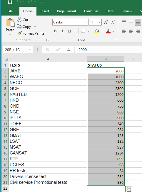
Select the range of cells, the table, or the whole sheet to that you want to apply conditional formatting to.

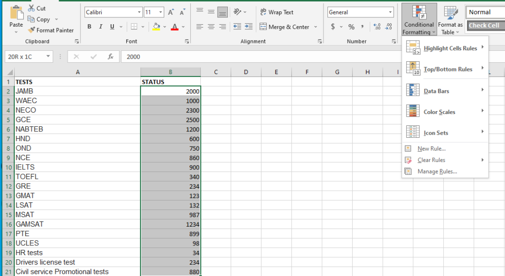
On the Home tab, click Conditional Formatting

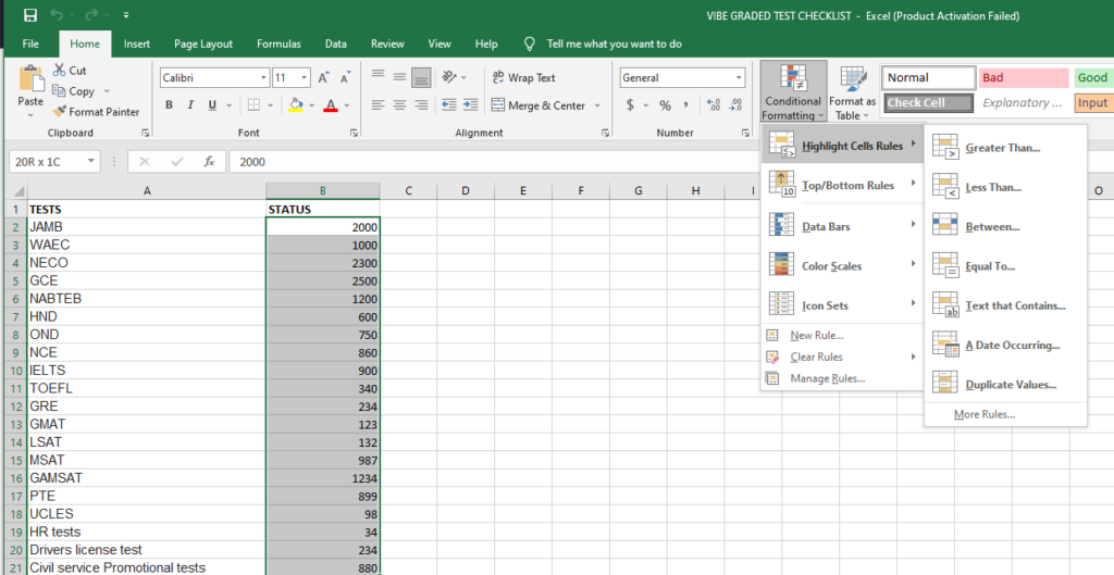
Point to Highlight Cells Rules, and then click Text that Contains.

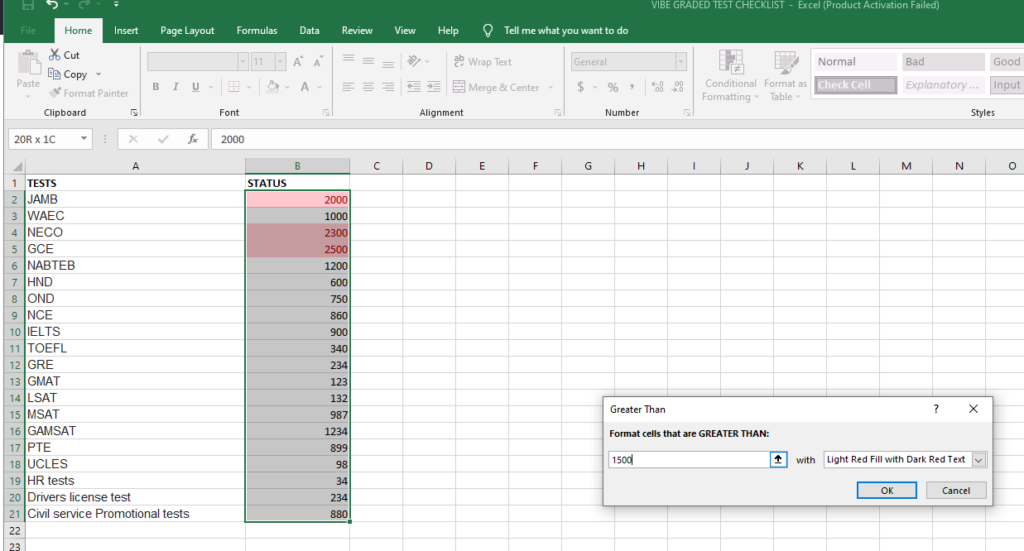
Type the text that you want to highlight, and then click OK

The process is slightly different if we are creating a custom conditional formatting rule.